Tutorial

Use Chunkflow as a Python Library

Chunkflow is a python library and all the operators can be used a python function. You can start using it with:

import chunkflow

For the full list of api functions, please checkout the API Reference.

Composable Command Line Interface

Chunkflow also provide a composable command line interface. You can compose operators and create your own pipeline flexibly for your specific application. The operators could be reused in different applications.

You can get a list of available operators by:

chunkflow

You’ll see a list like this:

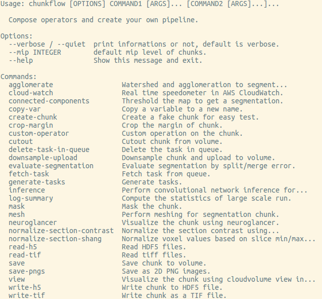
We keeps adding more and more operators, you might see more operators than this list. You can get help for each operator by typing chunkflow operator --help, such as:

chunkflow create-chunk --help

Now let’s play with some operators.

Visualization of a Chunk

Neuroglancer

create a random image volume and show it in neuroglancer:

chunkflow create-chunk neuroglancer

open the link and you should see it:

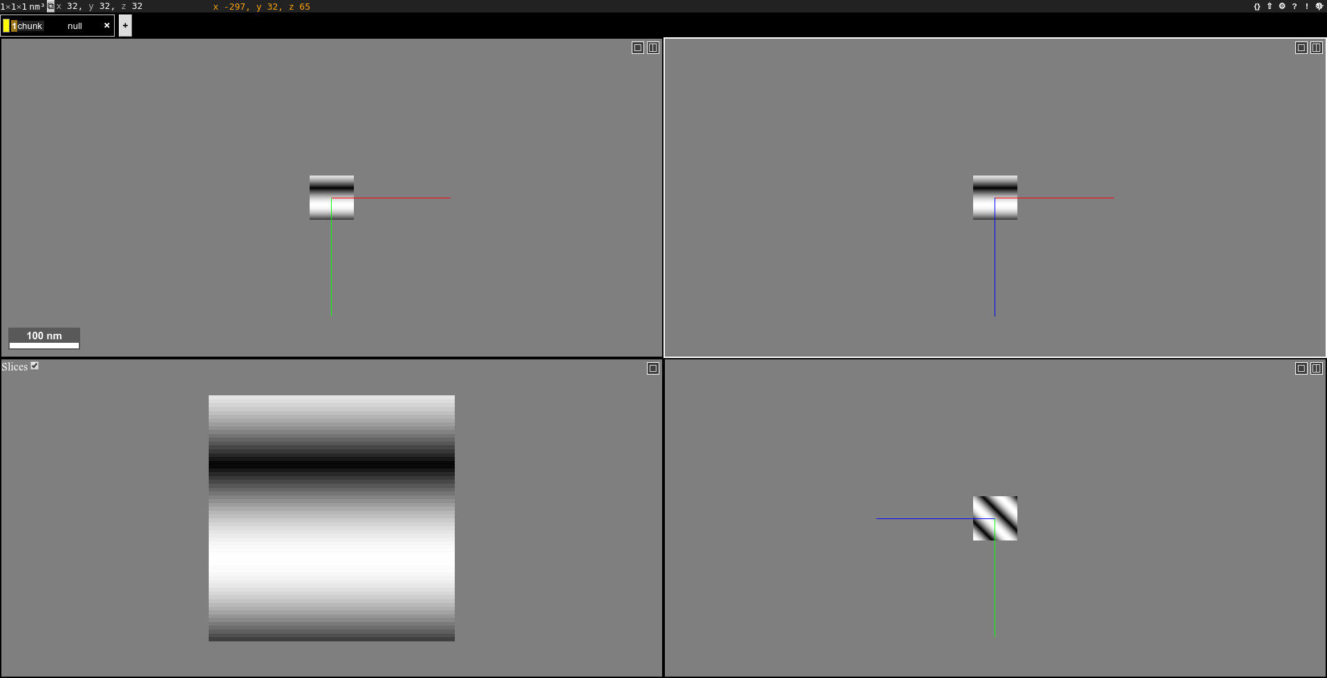
Note that the random image center is blacked out.

CloudVolume Viewer

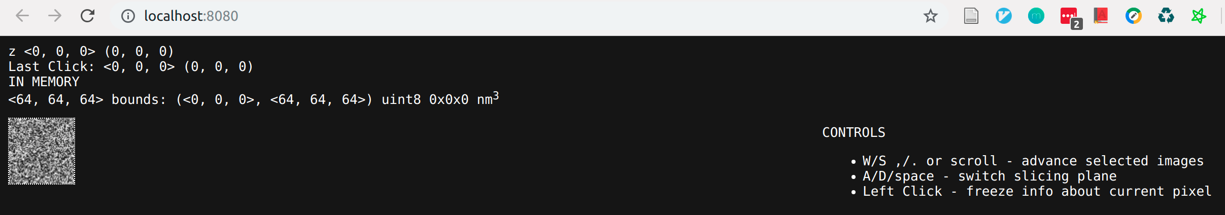
Create a random image volume and visualize it in browser:

chunkflow create-chunk view

open the link and you should see a image volume in browser:

Input and Output

I/O of Local Image

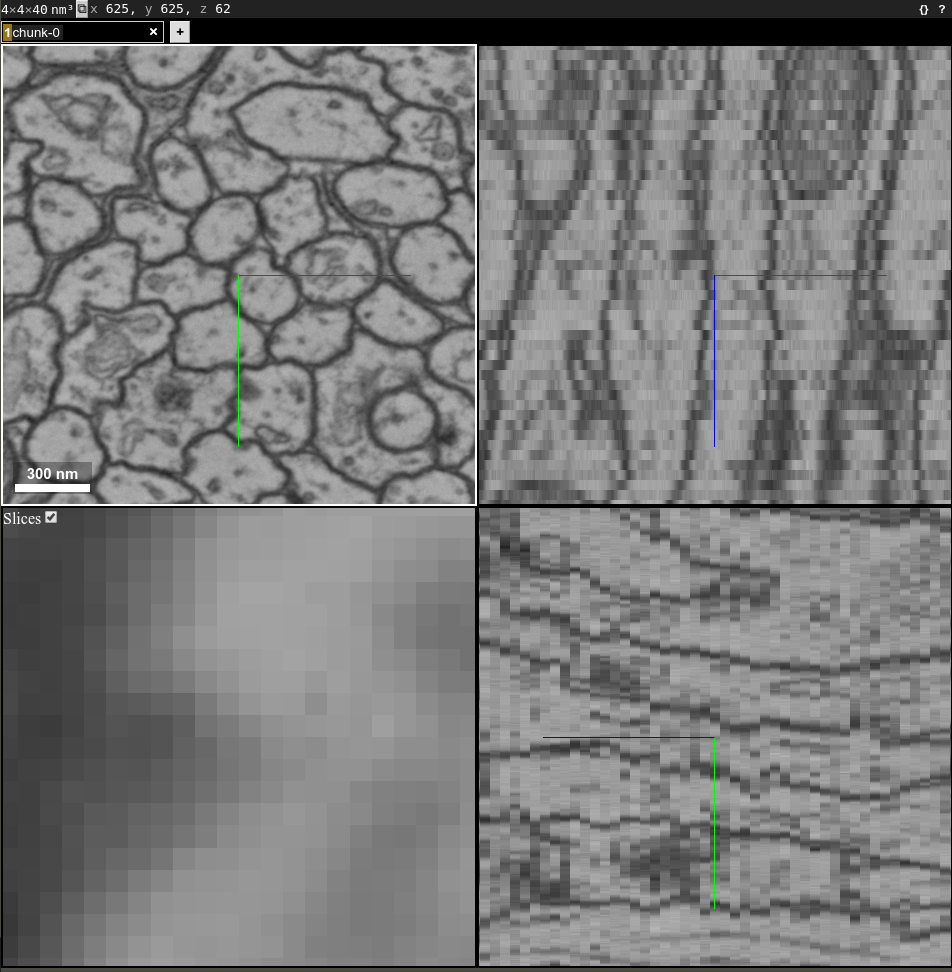
Now let’s play with some real data! You can download the data from CREMI challenge website. Let’s use the Dataset A for now.

Run this command and open the link in your browser:

chunkflow load-h5 --file-name sample_A_20160501.hdf --dataset-path /volumes/raw neuroglancer --voxel-size 40 4 4

Change the file path if you put your image in some other places. You should see the image in neuroglancer:

Cutout/Save a Chunk from Large Scale Volume in Cloud Storage

We use CloudVolume to perform cutout/saving of chunks in a large scale volumemetric dataset. To be convenient, we use local file system in this tutorial. To use cloud storage, you can just setup the authentication following the documentation of CloudVolume and replace the path to cloud storage. You can create a volume and ingest the image stack to the volume:

chunkflow load-h5 --file-name sample_A_20160501.hdf --dataset-path /volumes/raw save-precomputed --volume-path file:///tmp/your/key/path

Now you can cutout the image chunk from the volume:

chunkflow load-precomputed --volume-path file:///tmp/your/key/path --start 0 0 0 --stop 128 512 512 save-h5 --file-name /tmp/cutout_chunk.h5

Evaluation of Segmentation

You can read two segmentation volumes and compare them:

chunkflow load-tif --file-name groundtruth.tif -o gt load-tif --file-name /tmp/segmentation.tif -o seg evaluate-segmentation -g gt -s seg

The result will print out in terminal:

Rand split: 0.958776
Rand merge: 0.978602
VOI split: 0.300484
VOI merge: 0.143631

Of course, you can replace the load-tif operator to other reading operators, such as load-h5 and load-precomputed.

Convolutional Network Inference

Given a trained convolution network model, it can process small patches of image and output a map, such as synapse cleft or boundary map. Due to the missing context around patch boundary, we normally need to reweight the patch. We trust the central region more and trust the marginal region less. The inference operator performs reweighting of patches and blend them together automatically, so the input chunk size can be arbitrary without patch alignment. The only restriction is the RAM size. After blending, the output chunk will looks like a single patch and could be used for further processing.

We currently support multiple backends, including universal, pytorch and pznet. It is recommended to use the universal backend since it works universally. We load the source code dynamically. For an example, please take a look at our identity_backend.

Note

For pytorch backend, chunkflow will automatically use GPU for both inference and reweighting if there is GPU and cuda available.

In order to provide a universal interface for broader application, the ConvNet model should be instantiated, called InstantiatedModel, with all of it’s parameter setup inside. Chunkflow also provide a interface for customized preprocessing and postprocessing. You can define pre_process and post_process function to add your specialized operations. You can also define your own load_model function, and make some special loading operation, which is useful to load model trained with old version of pytorch (version<=0.4.0). This is an example of code:

def pre_process(input_patch):
   # we do not need to do anything,
   # just transfer input patch to net
   net_input = input_patch
   return net_input

def post_process(net_output):
   # the net output is a list of 5D tensor,
   # and there is only one element.
   output_patch = net_output[0]
   # the output patch is a 5D tensor with dimension of batch, channel, z, y, x
   # there is only one channel, so we drop it.
   # use narrow function to avoid memory copy.
   output_patch = output_patch.narrow(1, 0, 1)
   # We need to apply sigmoid function to get the softmax result
   output_patch = torch.sigmoid(output_patch)
   return output_patch

in_dim = 1
output_spec = OrderedDict(psd_target=1)
depth = 3
InstantiatedModel = Model(in_dim, output_spec, depth)

Note

If you do not define the pre_process and post_process function, it will automatically be replaced as identity function and do not do any transformation.

Synaptic Cleft Detection

With only one command, you can perform the inference to produce cleft map and visualize it:

chunkflow load-tif -f path/of/image.tif -o image inference --convnet-model model.py --convnet-weight-path weight.chkpt --patch-size 18 192 192 --patch-overlap 4 64 64 --framework pytorch --batch-size 6 --bump wu --num-output-channels 1 --mask-output-chunk -i image -o cleft save-tif -i cleft -f cleft.tif neuroglancer -c image,cleft -p 33333 -v 30 6 6

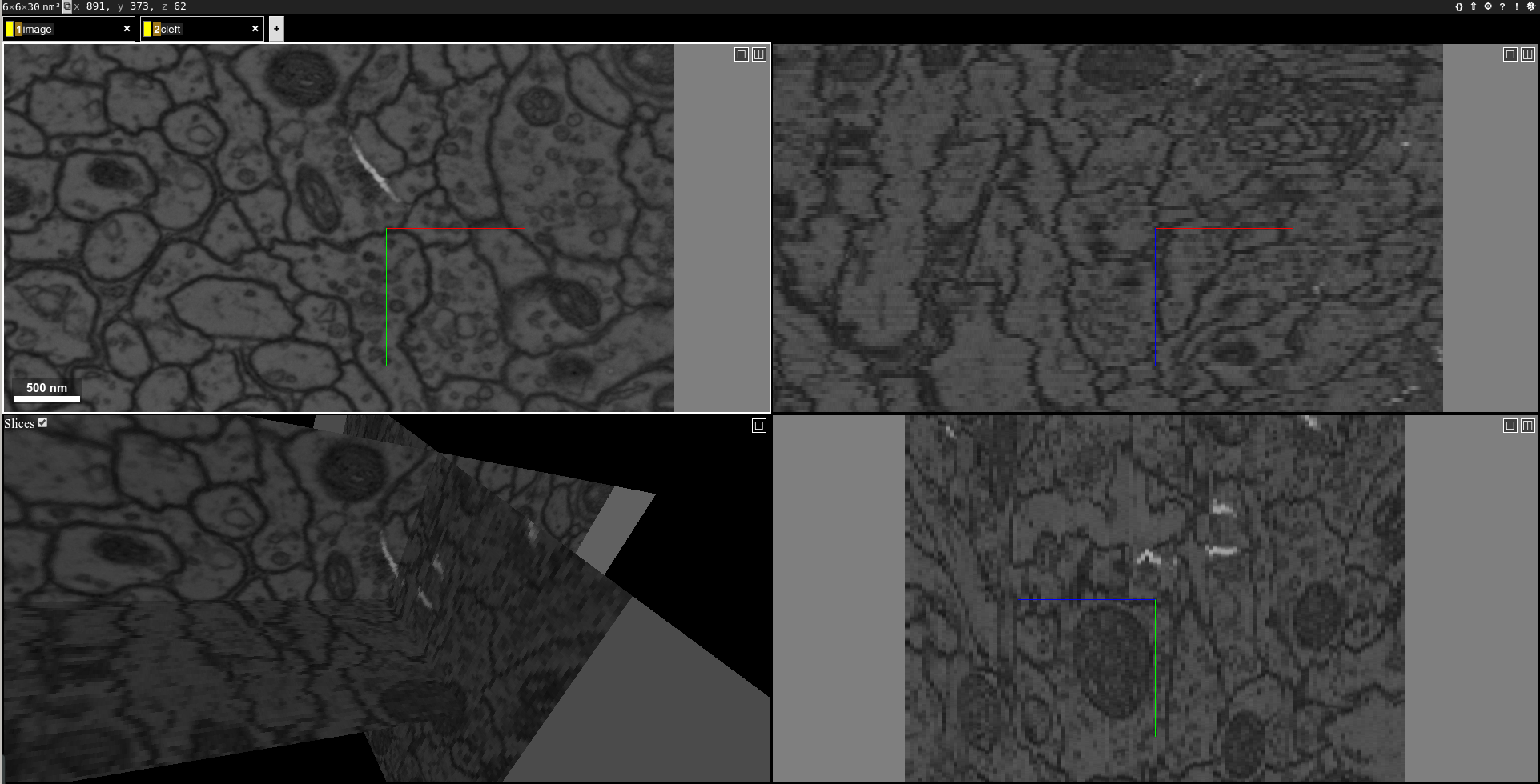
You can see the image with output synapse cleft map:

You can also apply a threshold to get a segmentation of the cleft map:

chunkflow load-tif -f path/of/image.tif -o image load-tif -f cleft.tif -o cleft connected-components -i cleft -o seg -t 0.1 neuroglancer -p 33333 -c image,seg -v 30 6 6

You should see segmentation overlayed with image:

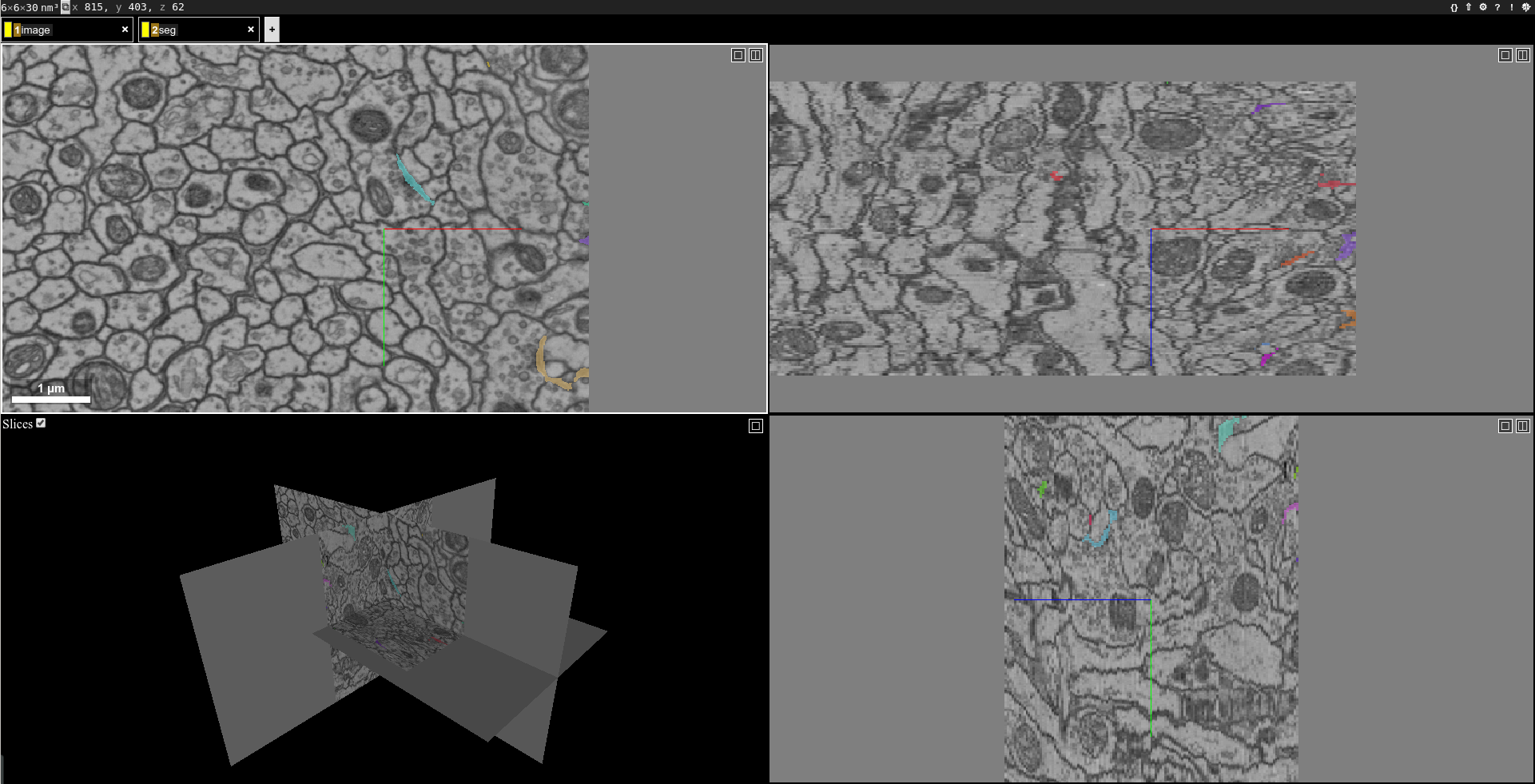
Of course, you can add a writing operator, such as save-tif, before the neuroglancer operator to save the segmentation.

Dense Neuron Segmentation

We used a ConvNet trained using SNEMI3D dataset, you can download the data from the website. Then, we can perform boundary detection with one single command:

chunkflow load-tif --file-name path/of/image.tif -o image inference --convnet-model path/of/model.py --convnet-weight-path path/of/weight.pt --patch-size 20 256 256 --patch-overlap 4 64 64 --num-output-channels 3 -f pytorch --batch-size 12 --mask-output-chunk -i image -o affs save-h5 -i affs --file-name affs.h5 neuroglancer -c image,affs -p 33333 -v 30 6 6

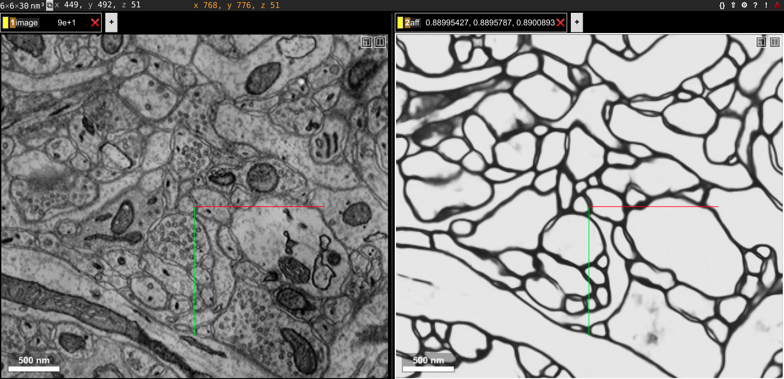
The boundary map is also saved in affs.h5 file and could be used in later processing. The affinitymap array axis is channel,z,y,x, and the channel order is x,y,z for our model output, meaning the first channel is x direction.

You can perform mean affinity segmentation with one single command:

chunkflow load-h5 --file-name affs.h5 -o affs agglomerate --threshold 0.7 --aff-threshold-low 0.001 --aff-threshold-high 0.9999 -i affs -o seg save-tif -i seg -f seg.tif load-tif --file-name image.tif -o image neuroglancer -c image,affs,seg -p 33333 -v 30 6 6

You should be able to see the image, affinity map and segmentation in neuroglancer. Overlay the segmentation with the image looks like this:

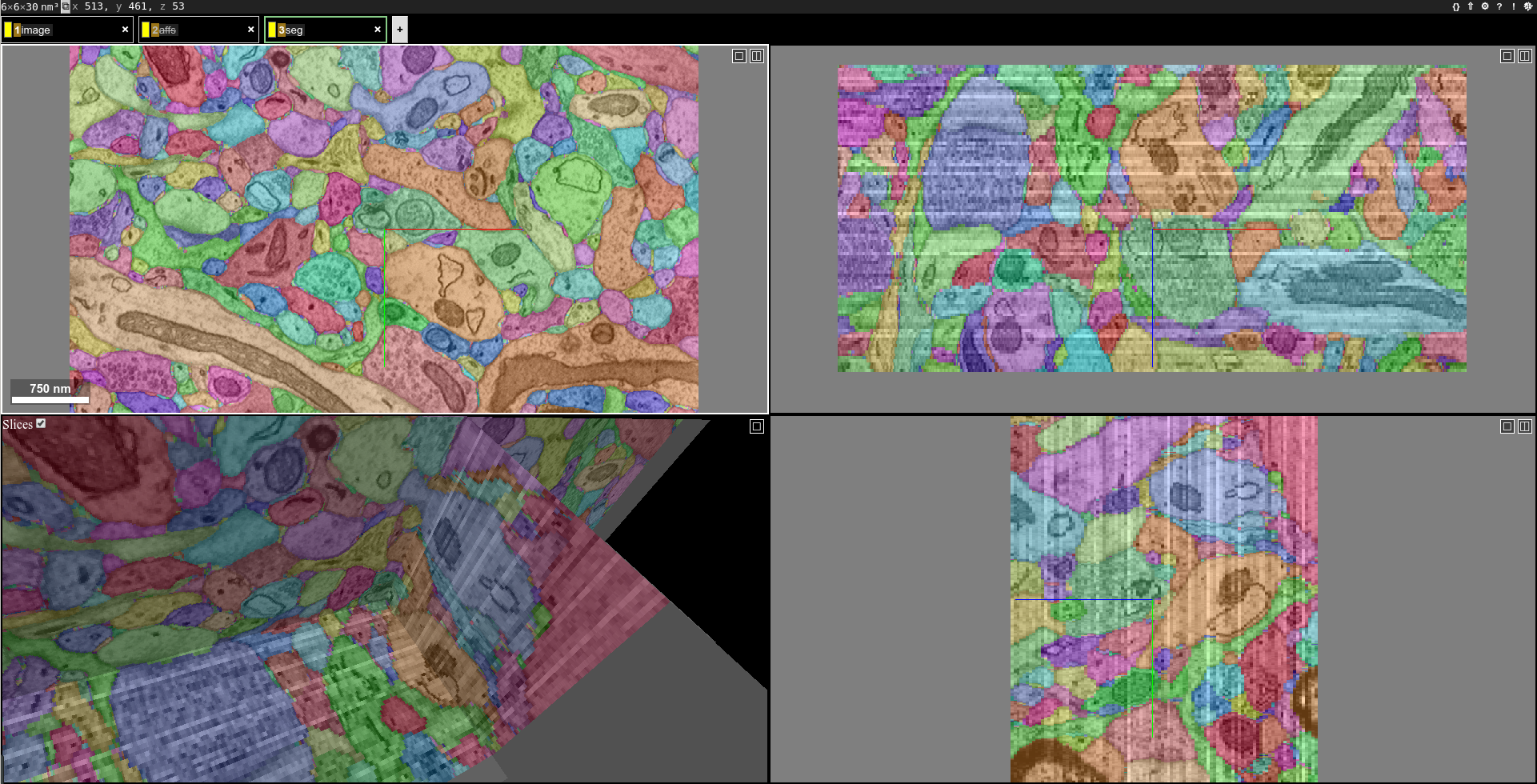
If the computation takes too long, you can decrease the aff-threshold-high to create bigger supervoxels or decrease the threshold to merge less watershed domains.

Of course, you can also combine the two setups to one single command:

chunkflow load-tif --file-name path/of/image.tif -o image inference --convnet-model path/of/model.py --convnet-weight-path path/of/weight.pt --patch-size 20 256 256 --patch-overlap 4 64 64 --num-output-channels 3 -f pytorch --batch-size 12 --mask-output-chunk -i image -o affs save-h5 -i affs --file-name affs.h5 agglomerate --threshold 0.7 --aff-threshold-low 0.001 --aff-threshold-high 0.9999 -i affs -o seg save-tif -i seg -f seg.tif neuroglancer -c image,affs,seg -p 33333 -v 30 6 6

Distributed Computation in Both Local and Cloud

We use AWS SQS queue to decouple task producing and managing frontend and the computational heavy backend. In the frontend, you can produce a bunch of tasks to AWS SQS queue, and the tasks are managed in AWS SQS. Then, you can launch any number of chunkflow workers in both local and cloud. You can even mix using multiple cloud instances. Actually, you can use any computer with internet connection and AWS authentication at the same time. This hybrid cloud architecture enables maximum computational resources usage.

Produce Tasks and Ingest to AWS SQS Queue

There are two ways of producing tasks, a smart way and a naive way.

Smart Way

It is recommended to use the smart way and all the parameters could be automatically calculated and computation environments setup. For example, you can use the following command to automatically calculate inference patch aligned output chunk size, create info metadata, including thumbnail, in cloud storage, and ingest tasks to AWS SQS queue.

chunkflow setup-env -l “gs://my-bucket/my/output/layer/path” -r 14 -z 20 256 256 -c 3 -m 1 –thumbnail -e raw -v 40 4 4 –max-mip 6 -q my-sqs-queue-name

Note

The output contains the parameters you need to use in later chunkflow command, such as patch number and output patch overlap.

This command will setup all the neccessary computational environment for the convolutional inference, you can then start your workers to consume the tasks in queue.

Naive Way

If you would like to control all the parameters your self, you can also use the generate-tasks to generate tasks directly with all your precalculated parameters. You have to setup the info files yourself. It will ingest the tasks to a AWS SQS queue if you define the queue-name parameter:

chunkflow generate-tasks --chunk-size 128 1024 1024 --grid-size 2 2 2 --stride 128 1024 1024 --queue-name my-queue

Log in your AWS console, and check the chunkflow queue, you should see your tasks there like this:

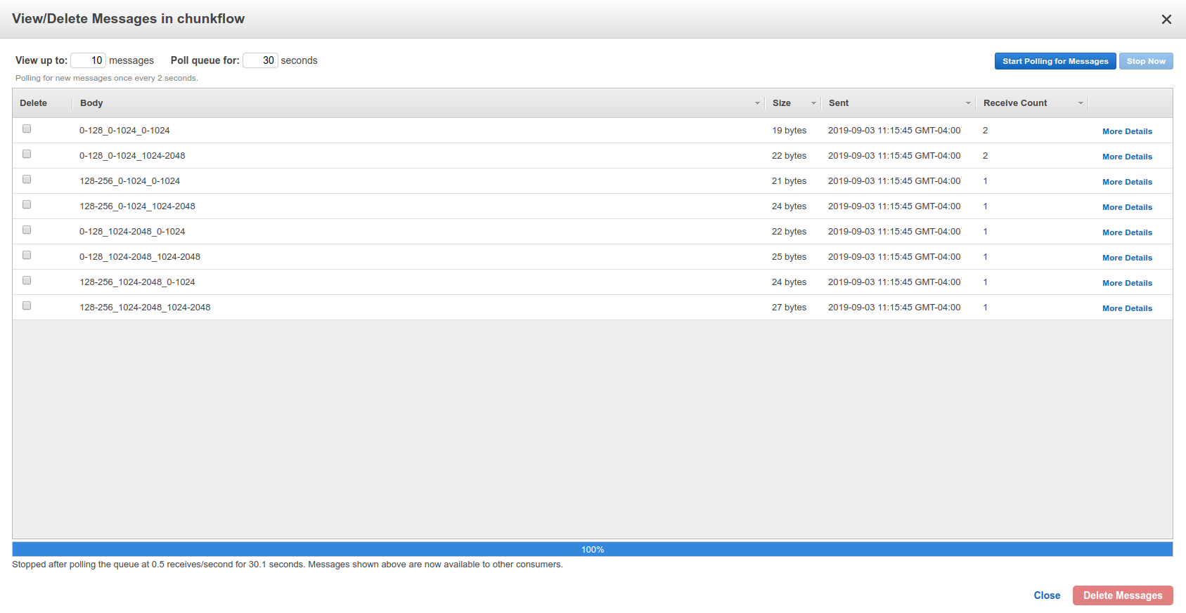
Chunkflow also provide a relatively smarter way to produce tasks using the existing dataset information. If you would like to process the whole dataset, we only need to define the mip level, and chunk size, all other parameters could be automatically computed based on the dataset information, such as volume start offset and shape. This is a simple example:

chunkflow generate-tasks -l gs://my/dataset/path -m 0 -o 0 0 0 -c 112 2048 2048 -q my-queue

Deploy in Local Computers

You can fetch the task from SQS queue, and perform the computation locally. You can compose the operations to create your pipeline.

Here is a simple example to downsample the dataset with multiple resolutions:

chunkflow --mip 0 fetch-task -q my-queue load-precomputed -v gs://my/dataset/path -m 0 --fill-missing downsample-upload -v gs://my/dataset/path --start-mip 1 --stop-mip 5 delete-task-in-queue

After downsampling, you can visualize the dataset with much larger field of view. Here is an example. Due to the limit of memory capacity of typical computers, we can not perform hierarchical downsampling from mip 0 to highest mip level in one step, thus we normally do in twice. For the first time, we perform downsampling from mip 0 to mip 5, than perform downsampling from mip 5 to mip 10.

Note

If you forget adding the delete-task-in-queue operator in the end, it will still works, but the task in queue will not be deleted and workers will keep doing the same task! This is good for debug, but not good in production.

Here is an example to generate meshes from segmentation in mip 3:

chunkflow --mip 3 fetch-task -q my-queue -v 600 load-precomputed -v gs://my/dataset/path --fill-missing mesh --voxel-size 45 5 5 -o gs://my/dataset/path --dust-threshold 100 delete-task-in-queue

The computation will also include a downsampling step for meshes to reduce the number of triangles. The meshing will produce chunked mesh fragments rather than the whole object mesh. Thus, we need another step, called mesh-manifest, to collect the fragments:

chunkflow mesh-manifest --volume-path gs://my/dataset/path --prefix 7

Normally, we have millions of objects in case of dense reconstruction of Electron Microscopy images. We would like to distribute the collection for speedup. We use prefix parameter to split the jobs. In the above example, we are only doing mesh manifest for objects start with 7. If all the object names start with number, we need to do it from 0 to 9, or from 00 to 99, to cover all the objects. The prefix will determine the number of jobs. If there are billions of objects, we might need to use deeper split, such as from 000 to 999. After the mesh manifest, you should be able to see the 3D objects using neuroglancer, like this one.

Note

This command will generate meshes for all the objects in the segmentation volume. You can also specify selected object ids using the –ids parameter. We normally call it sparse meshing. This is useful if you only need a few objects and will make the computation much faster.

Here is a complex example to perform convolutional inference:

chunkflow --mip 2 fetch-task --queue-name=my-queue --visibility-timeout=3600 load-precomputed --volume-path="s3://my/image/volume/path --expand-margin-size 10 128 128 --fill-missing inference --convnet-model=my-model-name --convnet-weight-path="/nets/weight.pt" --patch-size 20 256 256 --patch-overlap 10 128 128 --framework='pytorch' --batch-size=8 save-precomputed --volume-path="file://my/output/volume/path" --upload-log --nproc 0 --create-thumbnail cloud-watch delete-task-in-queue

Here is more complex example with mask and skip operations in production run of petabyte scale image processing:

export QUEUE_NAME="chunkflow"
export VISIBILITY_TIMEOUT="1800"
export IMAGE_volume_path="gs://bucket/my/image/layer/path"
export IMAGE_MASK_volume_path="gs://bucket/my/image/mask/layer/path"
export CONVNET_MODEL_FILE="model1000000.py"
export CONVNET_WEIGHT_FILE="model1000000.chkpt"
export OUTPUT_volume_path="gs://bucket/my/output/layer/path"
export OUTPUT_MASK_volume_path="gs://bucket/my/output/mask/layer/path"
export CUDA_VISIBLE_DEVICES="3"
chunkflow --mip 1 fetch-task -r 20 --queue-name="$QUEUE_NAME" --visibility-timeout=$VISIBILITY_TIMEOUT load-precomputed --volume-path="$IMAGE_volume_path" --expand-margin-size 10 128 128 --fill-missing mask --name='check-all-zero-and-skip-to-save' --check-all-zero --volume-path="$IMAGE_MASK_volume_path" --mip 8 --skip-to='save-precomputed' --fill-missing --inverse normalize-section-contrast -p "gs://bucket/my/histogram/path/levels/1" -l 0.0023 -u 0.01 inference --convnet-model="$CONVNET_MODEL_FILE" --convnet-weight-path="${CONVNET_WEIGHT_FILE}" --input-patch-size 20 256 256 --output-patch-size 16 192 192 --output-patch-overlap 2 32 32 --output-crop-margin 8 96 96 --num-output-channels 4 --framework='pytorch' --batch-size 6 --patch-num 14 9 9 mask --name='mask-aff' --volume-path="$OUTPUT_MASK_volume_path" --mip 8 --fill-missing --inverse save-precomputed --volume-path="$OUTPUT_volume_path" --upload-log --nproc 0 --create-thumbnail cloud-watch delete-task-in-queue

Note

The chunk size should also be divisible by the corresponding high mip level mask. For example, the chunk with size 24 x 24 x 24 can only be masked out with mip level no larger than 3. Because the maximum diviser of 24 with exponential of 2 is 8 (8=2^3). As a result, mask in high mip level will limit the chunk size choice!

For more details, you can checkout the examples folder in our repo.

For multiple processing in a single computer, you can use GNU Parallel to launch workers with a delay. For distributed processing in a local cluster, you can also use your cluster scheduler, such as Slurm Workload Manager, to run multiple processes and perform distributed computation.

Deploy to Kubernetes Cluster in Cloud

Kubernetes is the mainstay docker container orchestration platform, and is supported in almost all the public cloud computing platforms, including AWS, Google Cloud, and Microsoft Azure. You can use our template to deploy chunkflow to your Kubernetes cluster. Just replace the composed command you would like to use in the yaml file. For creating and managing cluster in cloud and usage, please check our wikipedia page.

To deploy using Kubernetes, you need to use docker image, which contains all the computational environments.

Build Docker Image

Automatic Update in Docker Hub

It is recommended to use Docker image for deployment in both local and cloud. Docker image contains all the computational environments for chunkflow and ensures that the operations are all consistent using the same docker image.

All the docker images are automatically built and is available in the DockerHub. The latest tag is the image built from the master branch. The base tag is a base ubuntu image, and the pytorch and pznet tag contains pytorch and pznet inference backends respectively. You can simply pull them and start using it:

sudo docker pull seunglab/chunkflow:latest

Manual Build Docker Image

If you modified the code and would like to manually build docker images locally. The docker files is organized hierarchically. The docker/base/Dockerfile is a basic one, and the docker/inference/pytorch/Dockerfile and docker/inference/pznet/Dockerfile contains pytorch and pznet respectively for ConvNet inference.

You can build the base image with:

cd docker/base
sudo docker build . -t seunglab/chunkflow:base --no-cache

Similarly, you can also build PyTorch base image:

cd docker/pytorch
sudo docker build . -t seunglab/chunkflow:pytorch --no-cache

After building the base images, you can start building chunkflow image with different backends. You can just modify the base choice in the Dockerfile and then build it:

# backend: base | pytorch | pznet | pytorch-cuda9
ARG BACKEND=pytorch

Then you can simply run:

sudo docker build . -t seunglab/chunkflow:latest --no-cache

Performance Analysis

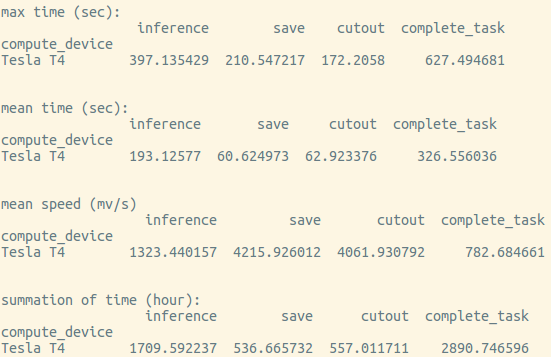
You can use log-summary to give a brief summary of operator performance:

chunkflow log-summary --log-dir /tmp/log --output-size 156 1280 1280

You should see the summary like this:

Add a New Plugin

Create a new python file with a function called execute. It is that simple, you can use your plugin now. Example usage could be found in the tests/command_lines.sh file. If you put your plugin file in the plugins folder, chunkflow will find it automaticaly, otherwise, you need to specify the exact path of your plugin in the --file parameter.

If you pass a chunk to your plugin and return a new chunk, the plugin function should look like as follows:

def execute(chunk: Chunk):
    ......
    return [chunk]

And then, you can use is like this:

chunkflow ...... plugin -f my_plugin -i chunk

If you pass more than one chunk to your plugin and return more than one chunk, the function should look like this:

def execute(chunk1: Chunk, chunk2: Chunk):
    ......
    return [chunk1, chunk2]

And then, you can use it as follows:

chunkflow ...... plugin -f my_plugin -i chunk1,chunk2 -o chunk1,chunk2

If you would like to pass some more arguments, you can encode the arguments as a string and decode it in your plugin. For example, you can encode your parameters as a JSON string and decode it using json. The plugin code would look like this:

def execute(chunk, args="some default parameters"):
    args = json.parse(args)
    ......
    return [chunk]

You can use it like this:

chunkflow ..... plugin -f my_plugin -i chunk --args "encoded parameter string"